Step 5 - Equilibrate the System
With our two processing layers set up we can start to run the simulation and monitor how the system is evolving. We’ll do this from the
page of the
 NeutronSQ module.
Go to the
RDF and Neutron S(Q) layer tab
Select the
We’ll visually compare the simulated total structure factor to the experimental one
Simulation ⇨ Run
You can also use
Ctrl-Rto start a simulation running
Note the counter towards the right-hand side of the status bar at the bottom of the main window which tracks the current iteration, and the status indicator to the far left of the status bar telling you what Dissolve is doing (and also note that pressing
Escstops the current simulation).
While the simulation is running you cannot edit any input values, keywords etc., but you can investigate the simulation’s progress and output as it happens. For example, you could go to the
Standard Atomic (MC/MD)
evolution layer and look at the
page of the
 Energy module to see what the total energy of the configuration is doing.
After the simulation has been running for a little while (perhaps 100 iterations), you’ll see that the calculated data compare quite favourably with the reference data, with the G(r) and F(Q) looking something like this:
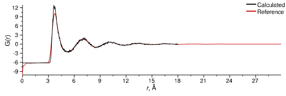
Equilibrated total G(r) for liquid argon
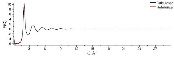
Equilibrated total F(Q) for liquid argon
When there is no further dramatic change in the calculated data you can stop the simulation:
Simulation ⇨ Stop
Or…
Esc
Keep in mind that the simulation will not actually stop until the current iteration is completed - most parts of the GUI will remain grayed out until then.