Step 5 - Assessing the Reference Potential
With our equilibrated (or equilibrating…) system we’ll now make a basic comparison between our simulated total structure factors and the reference datasets.
Go to the
G(r) / Neutron S(Q) tab
Click on the “H2O”
NeutronSQ module and select the Output button
We’ll first check the agreement between the experimental total structure factor (the F(Q)) and the simulated data. You’ll see a row of buttons at the top of the graph giving you access to various different plotted quantities, with the default being the which should look a little like this:
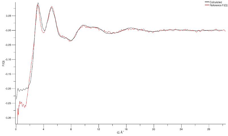
Calculated (black) and experimental (red) F(Q) for the equilibrated water (H2O) simulation
There are some small mismatches between the peak positions at $Q$ values of 3.1 and 5.1 Å-1 but overall the agreement is pretty good. The mismatch at $Q$ < 2 Å-1 is related to processing of the experimental data, and which we’ll not try to do anything to fix in this example.
Let’s take a look now at the total radial distribution functions:
Click the button on the “H2O”
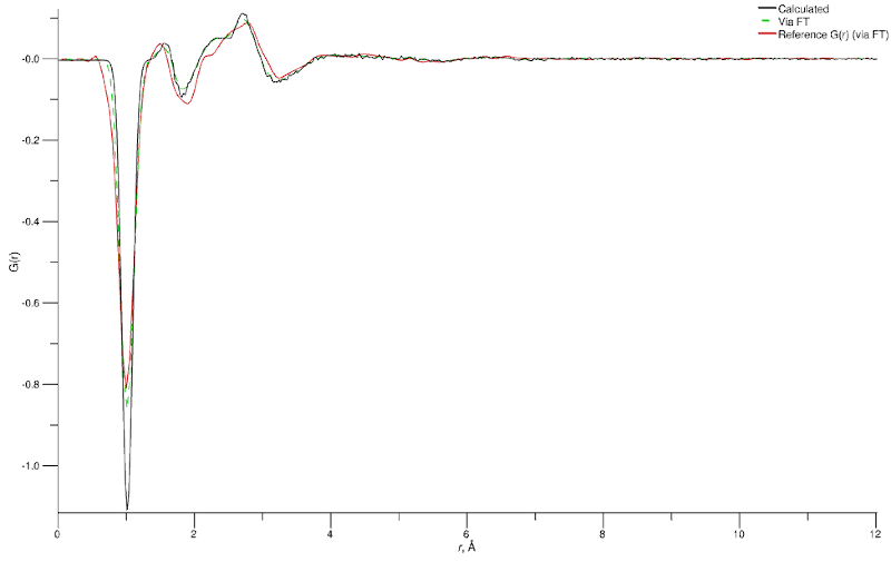
Simulated (black), Fourier-transformed from simulated F(Q) (green), and experimental (red) G(r) for the equilibrated water (H2O) simulation
On this graph you will have three curves which we’ll discuss individually as the distinctions are important.
Calculated G(r) (black)
The black line represents the G(r) calculated directly from the atomic coordinates in the configuration, with broadening applied to the intramolecular terms (if requested).
Experimental G(r) (red)
The experimental G(r) is obtained by Fourier-transforming the reference data and as such is a subject to all the potential artefacts introduced by doing so. A window function is typically applied, and the operational range of the Fourier transform is often truncated in order to reduce ripple effects or to avoid known “bad” data at the lower Q end of the spectrum.
Simulated G(r) Calculated by Fourier Transform (green)
Since the experimental data is subjected to Fourier transform in order to generate a reference G(r), the most reliable comparison to make is to simulated data treated in the same way. Thus, the green line (“Via FT” in the plot) is obtained by double Fourier of the original calculated G(r) (black line), taking it to Q-space and back again.
So, any critical comparison between simulated and experimental G(r) should be made by comparing the red and green lines.