Step 7 - Set up Potential Refinement
Let’s briefly recap what we’ve done so far:
- Set up a liquid water system based on a literature forcefield (
SPC/Fw, see http://dx.doi.org/10.1063/1.2136877) - Equilibrated the system and made an initial structural comparison with experimental data
- Adjusted the intramolecular geometry of the water molecule in order to better match the experimental data
Our agreement with experiment is relatively good, but it is possible to make it even better by modifying the inter-atomic interaction parameters contained in the atom types. However, generally this is not to be attempted by hand in all but the simplest of cases, as the effects of adjusting the interatomic are seldom as obvious as those for intra-molecular parameters. Also, for even a modestly-complicated system the number of adjustable parameters is simply too large to tackle with manual fitting.
Here we’ll employ the
 EPSR module in order to adjust the interatomic potentials automatically to give better agreement with the experimental reference data.
Esc
Layer ⇨ Create ⇨ Refinement ⇨ Standard EPSR
Our new layer contains only the
EPSR module, and which Dissolve has set up with sensible targets and defaults. We’ll explore the various graphs as we proceed, but for now let’s check the set-up of the module. Brief descriptions of the important parameters are given below - for more in-depth explanations see the
EPSR module page.
An initial value for EReq has been set (3.0) - this determines the magnitude or “strength” of the generated interatomic potentials
The Feedback factor is 0.9 - this states that we are 90% confident in the experimental data, and that the calculated partial structure factors should make up 10% of the estimated partials
The range of data over which to generate the potential in Q-space is determined by QMax (30 Å-1) and QMin (0.5 Å-1)
The experimental data to use in the refinement are set in the Target option, which lists all available modules by name that have suitable data for the EPSR module to use. You’ll see that Dissolve has added all of the available
 NeutronSQ modules have been selected automatically.
All of these default values are fine for our purpose, and there’s very little that you should have to change in the first instance. So, start the simulation running again to begin the refinement process:
Ctrl + R
While the simulation is running we’ll go through the different
tabs in the
EPSR module one by one to see what information we have available, and which help to illustrate the basic workflow of the EPSR methodology.
1. F(Q)
Basic comparison between reference experimental data (solid lines) defined as Targets and those simulated by Dissolve (dashed lines), including the difference functions (dotted lines).
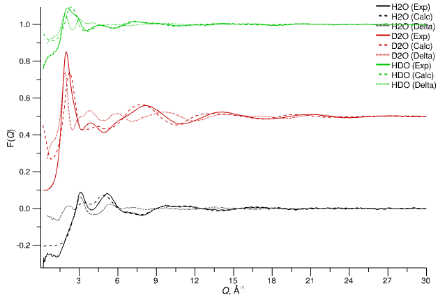
Experimental reference F(Q), calculated F(Q), and difference functions for data targeted by the EPSR module
2. Delta F(Q)
Delta functions between experiment and simulation are replicated here along with the fits to the functions achieved by the Poisson / Gaussian sums. Note that the difference functions here have been multiplied by -1.
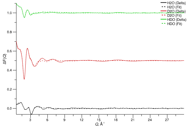
Delta functions (negated) and the Poisson/Gaussian fits to those functions
3. Estimated S(Q)
Estimated partial structure factors (solid lines) derived from combining experimental F(Q) and the calculated partial S(Q) (shown as dashed lines).
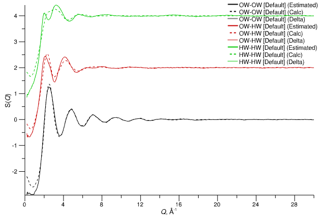
Estimated partial structure factors
4. Estimated g(r)
Partial radial distribution functions for each atom type pair in the system, showing estimated partials (solid lines, calculate by Fourier transform of the estimated S(Q)) and those from the simulation (dashed lines, calculated by Fourier transform of the simulated partial g(r)).
Note that the estimated g(r) from the combination of the experimental and simulated data are intermolecular partials - i.e. they contain no contributions from intramolecular terms related to the intramolecular bonding. The simulated partial g(r) (dashed lines), however, are the those calculated directly from the configuration(s) in the simulation, and include both intermolecular and intramolecular terms. The reason for this is to aid in detection of cases where the intramolecular structure of the molecules in the simulation is significantly different from that measured experimentally, which would manifest as small features in the estimated g(r) at or around the r-values associated to bond or angle (1,3) distances.
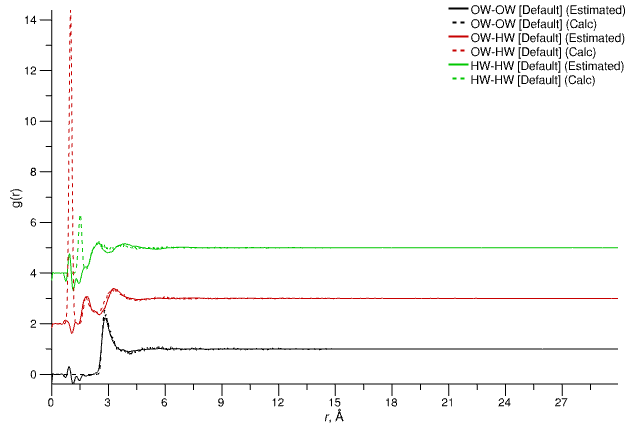
Estimated partial radial distribution functions
5. G(r)
Neutron-weighted total G(r) from Fourier transform of the reference F(Q) (solid line) and the Fourier transform of the simulated F(Q) (dashed line). As mentioned earlier, the reason for displaying the latter rather than the directly-calculated G(r) is to provide for a consistent comparison between simulation and experiment given the necessity of performing Fourier transforms (truncation errors are worse in Q-space data, so transforming to Q to r demands more judicious use of window functions in the transform).
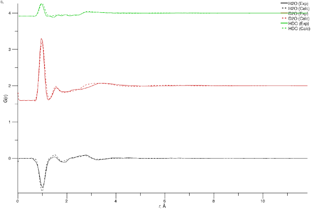
Total radial distribution functions from Fourier transform of reference and simulated F(Q) data
6. Potentials
φ(r) represent the empirical potentials generated from the difference data, one per pair potential. These are applied on top of the reference potential.
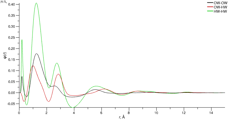
Empirical potentials for each atom type pair (i.e. each distinct pair potential)
7. R-Factors
For each experimental dataset the “goodness of agreement” with simulation is represented by the r-factor, along with the total (average) r-factor over all datasets.
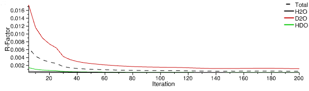
R-factors for experimental (reference) datasets
8. EReq
Here you can see the evolution of the current potential magnitude (whose limit is guided by the value of EReq).