Step 8 - Managing the Refinement
Now that our simulation is running and happily refining interatomic potentials, it’s fair to ask “How long should I refine for?”, or “What limit of EReq should I use?”, or even “How do I know when I’ve achieved the best agreement with experiment that I can get?”. The somewhat vague answer to all these questions is “When you can’t make the simulation any better.” Simply giving the
 EPSR module the freedom to do anything with a large EReq value is not a sensible approach, since it is highly likely that increasing the magnitude of the empirical potentials too much will harm the simulation rather than do it good. Unfortunately there is no direct way to determine what value of EReq is optimal a priori, and so some degree of trial and error is involved.
The EPSR algorithm implemented within Dissolve doesn’t contain any attempts at automating the adjustment of EReq, so a general procedure to follow is:
- Set a modest (i.e. low) value of EReq to begin with (the default of 3.0 is enough for neutral molecules, but should be higher for ionic systems).
- Run the simulation and observe the progression of the r-factors on the R-Factor tab of the module (hopefully they should decrease from their initial starting values).
- Once the r-factors have stabilised, increase EReq (increasing by an amount equivalent to the initial value each time is sensible).
- If the r-factors decrease again, repeat (3). If not, then you have probably reached the limit of what is possible within the context of the current simulation and its forcefield.
If you now take a look at the r-factors for your water simulation you should see that they have steadily decreased while you’ve been reading. In fact, an EReq value of around 3 represents the “limit of no improvement” for the present case - R-factors should be of the order of 1.4×10⁻⁴, and the simulated F(Q) should now agree pretty well with the experimental data:
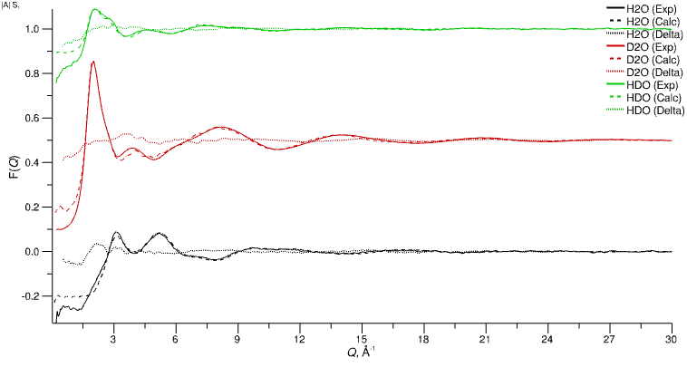
Experimental (solid lines) and simulated (dashed lines) total F(Q) after refinement
We can observe some discrepancies at the low Q end of the data, but there is little that we can do to remedy these errors since they are likely due to imperfect subtraction of inelasticity effects in the processing of the original data. Simulated F(Q) (even un-refined ones) often give a good indication of what the experimental data “should look like”, especially in the region where inelasticity effects dominate, and can be useful in guiding data processing (e.g. with Gudrun).
At this point, we can start to think about what kind of structural properties we want to calculate from our refined simulation.