Recommended Workflow

Standard Workflow?

Because of the scope and flexibility of Dissolve it isn’t possible to make a truly general recommendation on how it should be run. That said, the majority use case will be analysis of total scattering data according to the norms established by EPSR, so what follows here is the Dissolve take on performing such analyses. The overall message is to conduct your simulation in well-defined stages and save copies of the restart file after each one so that you can easily go back. There will be times where the need to restart your simulation from scratch is unavoidable, but that can be avoided on many occasions if restart files are captured and stored.

Set Up Your System

Obviously you first need to set up your system with the appropriate species, configuration, and layers. We’ll assume that for the latter you have something like the following:

• An Evolution layer which moves the stuff around in your system
• An RDF / SQ layer which calculates atomic partials and structure factors
• An EPSR layer to refine against the experimental data
• One or more Analysis layers to calculate something of interest

With all of this ready to go, the first step is equilibrating the system.

Equilibration

Typically, Dissolve will construct your initial configuration box from a defined generator procedure and which will most likely involve adding molecules at random positions and rotations. The first step is to equilibrate this high-energy system to a state where the energy is stable and there are no bad overlaps between atoms left in the system. The energy is of course completely defined by the forcefield you’ve used on your species, so we need to make a further assumption here that it is a reasonable forcefield!

For bulk liquid systems it is generally a good idea to apply a size factor to the box during these initial stages - this scales the box volume and the positions of the molecules, and greatly helps in the removal of overlapping molecules. You can find this option on the configuration tab, and a reasonable value to use is 10.

Evolution

To actually perform the equilibration you will want to turn off all layers except Evolution - you definitely don’t want to try refining or calculating properties while you’re equilibrating. In the GUI you can right-click on the Evolution tab and select Disable layers to the right, for example.

With that done, you can run your simulation for some number of steps. How many you will need to equilibrate the energy is heavily system dependent, ranging from a few hundred for a small-molecule liquid, to several thousand.

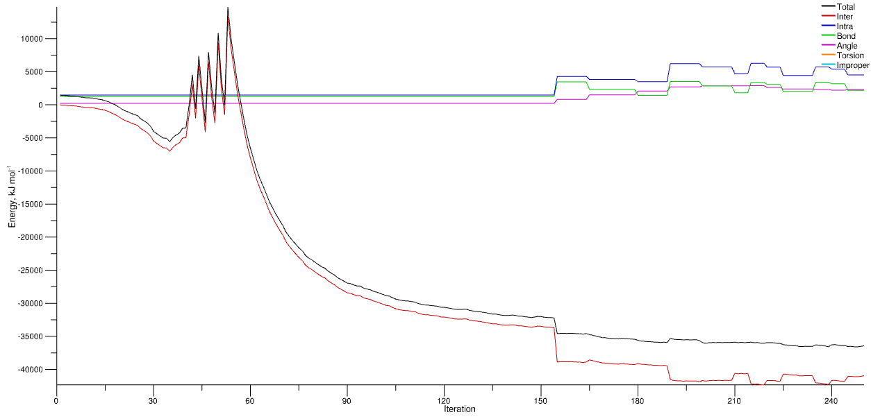
Evolution of energy from a random water configuration with size factor 10 applied at the outset. The spikes correspond to the sequential decreases of the size factor as the system relaxes and the molecules are gradually ‘compressed’ back to the requested density. At around step 160 the energy is stable enough for the MD module to kick in.

In the above graph you can see that the energy of the system has more-or-less stabilised by step 250, with the total energy fluctuating about a constant value. Note also that the interatomic energy (red line) - i.e. between molecules - is negative. This indicates a cohesive energy between the molecules which for a liquid means the simulation thinks it’s actually a liquid. A positive energy may indicate that the forcefield is incorrect, or that the density of the system is incorrect.

Evolution & RDF / SQ

Once your system has equilibrated it is worth calculating the initial correlation functions by enabling the RDF / SQ layer. You only need run for 25 - 50 steps in order to form the average with the default module settings.

Once that’s finish you should make a copy of the restart file and call it by an appropriate name (e.g. equilibrated.restart).

Refinement

The next thing to do is compare your calculated structure factors with any reference data you have supplied. If they look almost the same then congratulations - you can skip this section entirely! However this will not usually bee case, and there are two primary steps to take.

Molecule Geometry

The geometry of the molecules in your system is completely determined by the forcefield that you’ve applied, and it is entirely possible that you will find bond distances and angles in forcefields which do not agree with what is measured in reality. This is fair enough, since forcefields are typically not derived from experimental structural data, but you will need to correct them by hand as best you can. At present there is no reliable, automated way of achieving this, and the potentials applied by EPSR are interatomic and so cannot help correct imtramolecular terms.

You can determine quite quickly whether your bond and angle terms are consistent by comparing the total G(r) on, for example, your NeutronSQ module. If you see obvious mismatches in peak position you can adjust the relevant bond terms in your forcefield to try and get a better match. You can do a similar thing for slightly longer distances corresponding to the correlations between atoms at the end of angle terms.

There is of course a limit to this process, particularly with larger molecules where there may be many terms contributing to the same region in $r$, and even more so with angle terms. See the https://docs.projectdissolve.com/examples/water/ example for an illustration of the basic process.

Local Ordering

Now that your molecules “look” the best they can, the next step is to enable the EPSR module and try to fix the local ordering of those molecules. Generally you will start at a low value of ereq (the “power” which additional potentials have) and sequentially increase it in order to find the best value for your system. Again it will be system dependent, but the simulation might need to be run for several thousand steps. Before you change to a new value of ereq it is highly recommended to make a copy of the restart file (e.g. saving it to ereq3.restart for instance) since you will probably want to compare results and come back to what you consider to be the best value you discovered.

Analysis

Once you have settled on a value of ereq you can turn on any of your analysis layers and run for as long as you wish, or as long as is necessary to get good statistics on the properties of interest you’re targeting.